Declining real income in the US
I am not a big fan of income inequality per se as a policy issue. I care more about poverty alleviation and improving the living situation of the majority of Americans, versus capping the income or wealth of a segment of the population. Of course, there is an argument around concentration of power, and of heading off a course where we end up having the modern equivalent of a landed aristocracy, which I’m receptive to. But putting that aside for the moment, when I see graphs that show that income inequality is rising, I find myself thinking “that is a combination of two statistics, only one (the income of the average or lower-income segment of Americans) I really care about”.
So I decided to do a quick analysis, thinking it would show that income was rising across the board for all segments (even if income was rising faster in some segments vs. others, creating inequality). This is not what I found.
I took a sample of IPUMS data, which has individual-level data from the US census. I then built a series of smooth additive quantile regression models using the package qgam. (A quantile regression is where you’re estimating a conditional percentile, such as the median — 50th percentile — or some other, like 90th or 10th, as opposed to the mean. Smooth and additive = think generalized additive model).
I then regressed the individual-level income data on the year, age of the respondent, and the sex of the respondent. Here are the graphs of the year coefficient for the 10th, 50th, and 90th percentiles:
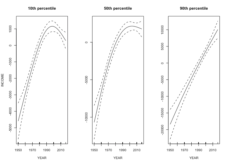
Basically, the largest incomes have kept increasing. The median income has stagnated from sometime between 1990 and 2000. And worst of all, the lower incomes have declined to roughly 1980 levels in the past 20 years.
Now, this isn’t the same thing as saying the income of the wealthiest Americans have kept increasing — people’s incomes change quite a bit from year to year — but it is true to say that if you happen to find yourself in the 10th percentile of incomes in a given year, you’re going to be earning substantially less than you would have been in 2000. That is a Bad Thing.
# from IPUMS
# includes 1950 forward
# includes individual income
# sex
# age

raw_data <- data.table::fread("~/Downloads/usa_00008.csv")

library(tidyverse)
includes_income <- raw_data %>%
  filter(!is.na(INCTOT)) %>%
  filter(INCTOT != 9999999) %>%
  filter(INCTOT != -000001) %>%
  filter(INCTOT != -009995)


# http://www.in2013dollars.com/us/inflation/1950
adjusted_income <-
  includes_income %>%
  mutate(
    ADJINC = case_when(
      YEAR == 1950 ~ INCTOT * 10.49,
      YEAR == 1960 ~ INCTOT * 8.54,
      YEAR == 1970 ~ INCTOT * 6.51,
      YEAR == 1980 ~ INCTOT * 3.07,
      YEAR == 1990 ~ INCTOT * 1.93,
      YEAR == 2000 ~ INCTOT * 1.47,
      YEAR == 2010 ~ INCTOT * 1.16,
      YEAR == 2017 ~ INCTOT * 1.03
    )
  ) %>%
  mutate(ADJYEAR = YEAR - 1950)

library(mgcv)
library(qgam)

mod_05 <- qgam(ADJINC ~ s(YEAR, k = 4) + s(AGE) + factor(SEX), # weight
               data = sample_n(adjusted_income, 10000, weight = PERWT, replace = T), qu = 0.05)

mod_10 <- qgam(ADJINC ~ s(YEAR, k = 4) + s(AGE) + factor(SEX), # weight
             data = sample_n(adjusted_income, 10000, weight = PERWT, replace = T), qu = 0.1)

mod_50 <- qgam(ADJINC ~ s(YEAR, k = 4) + s(AGE) + factor(SEX), # weight
               data = sample_n(adjusted_income, 10000, weight = PERWT, replace = T), qu = 0.5)

mod_90 <- qgam(ADJINC ~ s(YEAR, k = 4) + s(AGE) + factor(SEX), # weight
               data = sample_n(adjusted_income, 10000, weight = PERWT, replace = T), qu = 0.9)

mod_95 <- qgam(ADJINC ~ s(YEAR, k = 4) + s(AGE) + factor(SEX), # weight
               data = sample_n(adjusted_income, 10000, weight = PERWT, replace = T), qu = 0.95)


par(mfrow = c(1,3))
mod_10 %>% plot(scale = 0, select = 1, main = "10th percentile", ylab = "INCOME")
mod_50 %>% plot(scale = 0, select = 1, main = "50th percentile", ylab = "")
mod_90 %>% plot(scale = 0, select = 1, main = "90th percentile", ylab = "")
par(mfrow = c(1,1))

par(mfrow = c(1,2))
mod_05 %>% plot(scale = 0, select = 1, main = "5th percentile", ylab = "INCOME")
mod_95 %>% plot(scale = 0, select = 1, main = "95th percentile", ylab = "")
par(mfrow = c(1,1))